The Back Propagation Algorithm

Artificial Neural Networks

Artificial Neural Networks (ANNs) are loosely modeled after the brain. ANNs are composed of units (also called nodes) that are modeled after neurons, with weighted links interconnecting the units together.

What ANN?

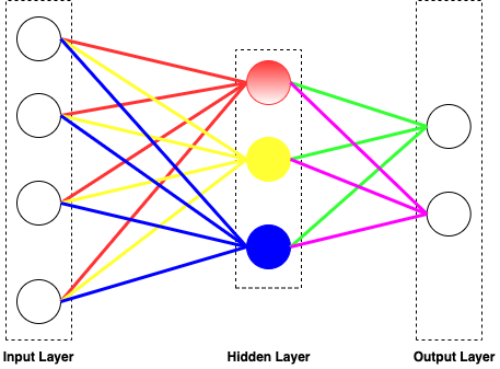
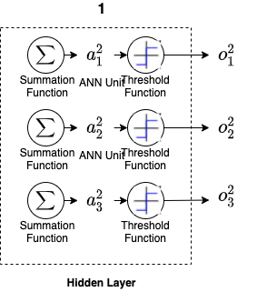
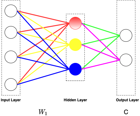
Overall, the ANN contains input layer, hidden layer and the output layer.

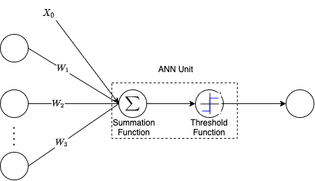
Each hidden layer has an input, an output and a number of ANN units while the ANN unit is composed of two main parts: the first part sums the input and sends it to the threshold function.

If the activation is greater than 0 then the unit activates and sends a “1” as the output, otherwise it sends a 0 (or –1). The $X_0$ can be set to any value so that instead of tuning the threshold function to activate at some fixed point Y, X0 can be set to -Y.

Why ANN?

Can approximate any function(when target function is not known)
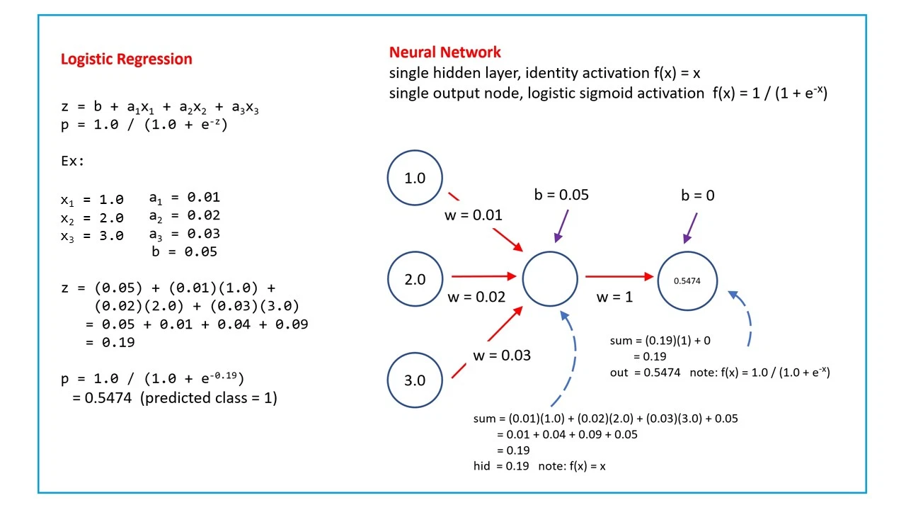
Is a superset of a logistic regression(when output is a vector of continuous or discrete values)

Forward Propagation

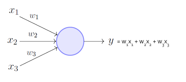
Let’s take one ANN unit out from the ANN. From the defintion, an ANN unit is a composition of a summation function and a threshold function(a.k.a activation function). Before describing the forward propagation, let’s define some terms and defintions.

Threshold Function

For each ANN unit, the summation result will be passed to a thresold function for an output. Let’s say $a_i^k$ is the $i^{th}$ input in the $k^{th}$ layer and the corresponding output is $o_i^k$ . Below is an example of input and output in layer #2

A vector can be used to describe all scalar input/output in the same layer.

a_k = \left[ \begin{matrix} a_1^k \\ a_2^k \\ a_3^k \end{matrix} \right], o_k = \left[ \begin{matrix} a_1^k \\ a_2^k \\ a_3^k \end{matrix} \right]

Applying the same threshold function $f$ to all inputs in the same layer will give us the relationship between input and output.

o_k = \left[ \begin{matrix} a_1^k \\ a_2^k \\ a_3^k \end{matrix} \right] = \left[ \begin{matrix} f(a_1^k) \\ f(a_2^k) \\ f(a_3^k) \end{matrix} \right] = f(\bm{a_k})

Then we have our first formula,

o_k = f(\bm{a_k}) \tag{1}

Weights and Summation

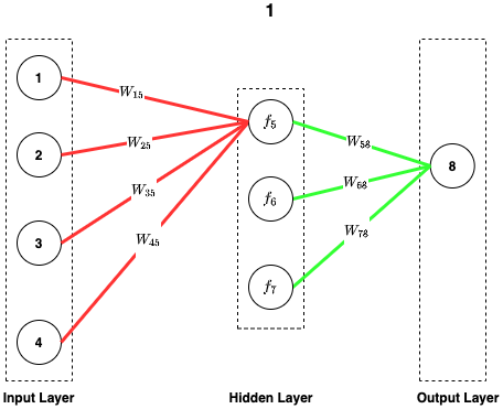
Weight is the connection between each layer and its previous layer. Below is an example of weights in a 3-layer ANN.

If we’d like to calculate the input of node #5, we will need to sum up four input node with its weight. Let’s say $o_i$ is the $i_{th}$ input node, $w_{i5}$ is the weigth between node #1 and #5.

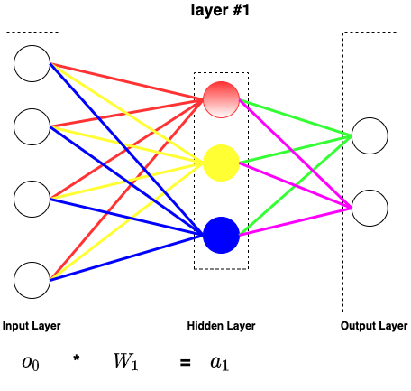
a_5 = w_{15} * o_1 + w_{25} * o_2 + w_{35} * o_3 + w_{45} * o_4 = \left[ \begin{matrix} w_{15}, w_{25}, w_{35}, w_{45} \end{matrix} \right] * \left[ \begin{matrix} o_1 \\ o_2 \\ o_3 \\ o_4 \end{matrix} \right]

Put all nodes in the layer#1 together will give us a more complex matrix expression. Take $o_0$ as input, $a_1$ be the output of the summation(input to threshold function in layer #1)

\bm{a_1} = \left[ \begin{matrix} w_{15} * o_1^0 + w_{25} * o_2^0 + w_{35} * o_3^0 + w_{45} * o_4^0 \\ w_{16} * o_1^0 + w_{26} * o_2^0 + w_{36} * o_3^0 + w_{46} * o_4^0 \\ w_{17} * o_1^0 + w_{27} * o_2^0 + w_{37} * o_3^0 + w_{47} * o_4^0 \\ \end{matrix} \right] = \left[ \begin{matrix} w_{15}, w_{25}, w_{35}, w_{45} \\ w_{16}, w_{26}, w_{36}, w_{46} \\ w_{17}, w_{27}, w_{37}, w_{47} \\ \end{matrix} \right] * \left[ \begin{matrix} o_1^0 \\ o_2^0 \\ o_3^0 \\ o_4^0 \end{matrix} \right] = \bm{W_1} * \bm{o_0}

Every layer follows the same pattern, then we have our second formula,

Define $W_k$ be the weight matrix of $k^{th}$ layer, $\bm{o_{k-1}}$ be the output from the previous layer, and $\bm{a_k}$ be the output of summation(input to layer #k)

\bm{W_k}*\bm{o_{k-1}} = \bm{a_k} \tag{2}

Forward Propagation Algorithm

Let’s have a quick recap on two important formula from the previous section,

o_k = f(\bm{a_k}) \tag{1}

\bm{W_k}*\bm{o_{k-1}} = \bm{a_k} \tag{2}

The formula #1 changes $\bm{a}$ to $\bm{o}$ while formula #2 push result to the next layer.

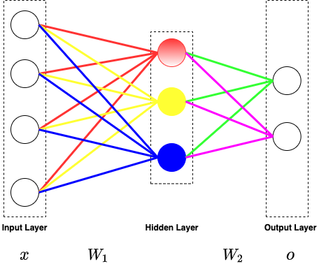
With the input $\bm{x}$ and the weight matrix $\bm{W}$ , we can calculate the output easily by using formula #1 and formula #2

\bm{o} = f(\bm{W_2}f(\bm{W_1}\bm{x})

Back Propagation

The back propagation is an algorithm to update the weight in order to minimize the difference between the expected output and the actual output from forward propagation in the training set.

Goal

Let’s define loss function first. Usually we use distance between expected output and the actual output. Say that $\bm{o}$ is the output calculated from forward propagation while $\bm{y}$ is the expected output from the training set.

C = \frac{1}{2}(\bm{o} - \bm{y})^2

Our goal is to minimize the C by updating $\bm{W}$ in each layer. What we usually do is gradient descent.

\bm{W_k} = \bm{W_k} - \eta \frac{\partial C}{\partial \bm{W_k}} \tag{3}

The question is how to find the connection of $W_1$ with $C$ (and $W_2$ with $C$ )

Chain Rule

Since C is the function of $\bm{o}$ , $C = \frac{1}{2}(\bm{o} - \bm{y})^2$ , $\bm{o}$ is the function of $\bm{a}$ , $o_k = f(\bm{a_k})$ and $\bm{a}$ is the function of $\bm{W}$ , $\bm{W_k}*\bm{o_{k-1}} = \bm{a_k}$ , we can transfer the partial derivative of $C$ with $W$ into with $\bm{a}$ by chain rule.

\frac{\partial C}{\partial \bm{W_k}} = \frac{\partial C}{\partial \bm{a_k}} \frac{\partial a_k}{\partial \bm{W_k}}

From formula {2}, $\bm{W_k}*\bm{o_{k-1}} = \bm{a_k}$

\frac{\partial a_k}{\partial \bm{W_k}} = \frac{\partial \bm{W_k} * \bm{o_{k-1}}}{\partial \bm{W_k}} = \bm{o_{k-1}}^T

The next step is to find out $\frac{\partial C}{\partial \bm{a_k}}$

Error Term

Let’s define error term as

\epsilon_k = \frac{\partial C}{\partial \bm{a_k}}

It doesn’t seem like we can calculate $\epsilon_k$ directly, but what if we know $\epsilon_{k+1}$

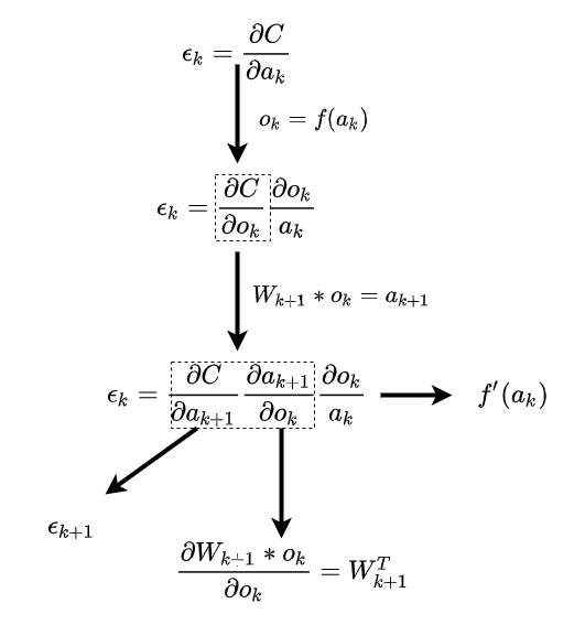
From formula #1 and #2,

o_k = f(\bm{a_k}) \tag{1}

\bm{W_{k+1}}*\bm{o_{k}} = \bm{a_{k+1}} \tag{2}

we can transfer our original task to the following equation by chain rule

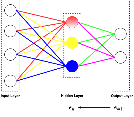
Back Propagation Algorithm

The BP algorithm is calculated in a reverse direction compared to the forward propagation. The algorithm is described as follows,

For each layer $k$ from the right to left,

calculate the error term by the error rate of $k + 1$ layer.

\epsilon_k = \epsilon_{k+1}W_{k+1}^Tf'(a_k)

The rightmost layer(output layer) error term, y’ is the actual output while y is the expected output

\epsilon = (y' - y)f'(a_k)

update the weights by the error term and output of $k$ layer

\bm{W_k} = \bm{W_k} - \eta\epsilon_ko_k

XOR Problem

The XOr, or “exclusive or”, problem is a classic problem in ANN research. It is the problem of using a neural network to predict the outputs of XOr logic gates given two binary inputs. An XOr function should return a true value if the two inputs are not equal and a false value if they are equal.

Traning Set

All possible inputs and predicted outputs are shown below.

Input 1	Input 2	Output
0	0	0
0	1	1
1	0	1
1	1	0

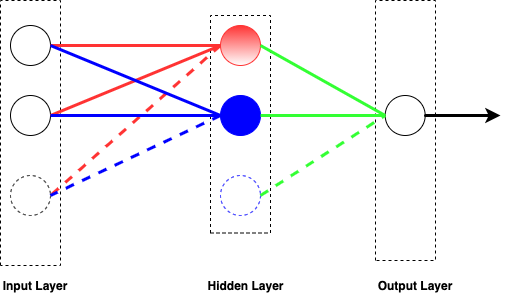
Traning ANN

2 dimensional inputs with 1 dimensional output(binary classification) and 1 hidden layer with 2 ANN units.

Implementation

def tanh(x):
    return np.tanh(x)


def tanh_derivative(x):
    return 1 - np.tanh(x) * np.tanh(x)


def logistic(x):
    return 1 / (1 + np.exp(-x))


def logistic_derivative(x):
    return logistic(x) * (1 - logistic(x))


class NeuralNetwork:
    def __init__(self, layers, activation='logistic', la=0):
        if activation == 'logistic':
            self.activation = logistic
            self.activation_deriv = logistic_derivative
        elif activation == 'tanh':
            self.activation = tanh
            self.activation_deriv = tanh_derivative

        self.weights = []
        self.regularization = Regularization(la)
        for i in range(1, len(layers) - 1):
            # Return random floats in the half-open interval [-0.25, 0.25]
            self.weights.append((2 * np.random.random((layers[i - 1] + 1, layers[i] + 1)) - 1) * 0.25)
        self.weights.append((2 * np.random.random((layers[i] + 1, layers[i + 1])) - 1) * 0.25)

    def fit(self, x_train_mat, y_train_mat, learning_rate=0.02, epochs=20000):
        """ gradient for linear regression
           Parameters
           ----------
           x_train_mat: matrix
           y_train_mat: array
           learning_rate: matrix in n * 1
               n features
           epochs:
        """
        x_train_mat = NeuralNetwork.append_ones_at_last(x_train_mat)
        self._gradient_descent(x_train_mat, y_train_mat, learning_rate, epochs)

    def predict(self, x_predict_mat):
        x_predict_mat = NeuralNetwork.append_ones_at_last(x_predict_mat)
        a = NeuralNetwork.feed_forward(self.weights, x_predict_mat, self.activation)

        return a[-1]

    @staticmethod
    def cost_function(weights, x_train_mat, y_train_mat, activation):
        a = NeuralNetwork.feed_forward(weights, x_train_mat, activation)

        return np.dot((y_train_mat - a[-1]).T, (y_train_mat - a[-1]))[0, 0]

    @staticmethod
    def feed_forward(weights, x_train_mat, activation):
        a = [x_train_mat]

        for l in range(len(weights)):
            a.append(activation(np.dot(a[l], weights[l])))

        return a

    @staticmethod
    def deltas(weights, a, m, y_train_mat, activation_deriv, regularization):
        error = y_train_mat - a[-1]
        deltas = [error * activation_deriv(a[-1])]
        for l in range(len(a) - 2, 0, -1):
            gradient = np.multiply(deltas[-1].dot(weights[l].T), activation_deriv(a[l]))
            regular_term = regularization.regularization_term_gradient(m, weights[l])
            deltas.append(gradient + regular_term.T)

        deltas.reverse()

        return deltas

    def _gradient_descent(self, x_train_mat, y_train_mat, learning_rate=0.2, epochs=20000):
        m = x_train_mat.shape[0]
        loss_list = []
        epochs_list = []
        for k in range(epochs):
            i = np.random.randint(x_train_mat.shape[0])
            a = NeuralNetwork.feed_forward(self.weights, x_train_mat[i], self.activation)
            cost = NeuralNetwork.cost_function(self.weights, x_train_mat, y_train_mat, self.activation)
            loss_list.append(cost)
            epochs_list.append(k)
            deltas = NeuralNetwork.deltas(self.weights, a, m, y_train_mat[i],
                                          self.activation_deriv, self.regularization)

            for i in range(len(self.weights)):
                layer = np.atleast_2d(a[i])
                delta = np.atleast_2d(deltas[i])
                self.weights[i] += learning_rate * layer.T.dot(delta)

        plt.plot(epochs_list, loss_list)
        plt.xlabel('epochs')
        plt.ylabel('loss')
        plt.show()

    @staticmethod
    def append_ones_at_last(x_train_mat):
        temp = np.ones([x_train_mat.shape[0], x_train_mat.shape[1] + 1])
        temp[:, 0:-1] = x_train_mat
        return temp

0,0,0
0,1,1
1,0,1
1,1,0

def test_xor(data):
    x_train_mat = data[0]
    y_train_mat = data[1]
    nn = NeuralNetwork([2, 2, 1], 'tanh')
    nn.fit(x_train_mat, y_train_mat)
    test_cases = [([0, 0], 0), ([0, 1], 1), ([1, 0], 1), ([1, 1], 0)]
    for test_case in test_cases:
        np.testing.assert_almost_equal(test_case[1], nn.predict(np.asmatrix(test_case[0])), decimal=1)

Shawn's Blog